站点设定

仓库
语言设定
货币设定
资源
视频库
Cx Family Common Mode Chokes
0402CT Low Profile Chip Inductors
XAL7050 High-inductance Shielded Power Inductors

XGL4020 Ultra-low DCR Power Inductors

Transformer Model Considerations

Simulation Model Considerations: Part II

Choose or Create Meaningful Power Transformer Models for SPICE Simulations

In Part I of this series, we discussed the challenges and limitations of modeling inductors in SPICE, which included examples of how to select the appropriate inductor model for various types of simulations. We then explored the variety of Coilcraft inductor models for meaningful simulations in each type of application. In Part II, we will extend the discussion to challenges and limitations of modeling transformers in SPICE and how to overcome these challenges.

Transformer SPICE models are intended to be virtual representations that behave in simulations like real transformers do in physical circuits. For this to be true, models must be designed carefully to capture all the appropriate characteristics of the transformer. Furthermore, the simulation may give the wrong impression if it is being used to verify operating conditions other than those originally intended by the model creator.

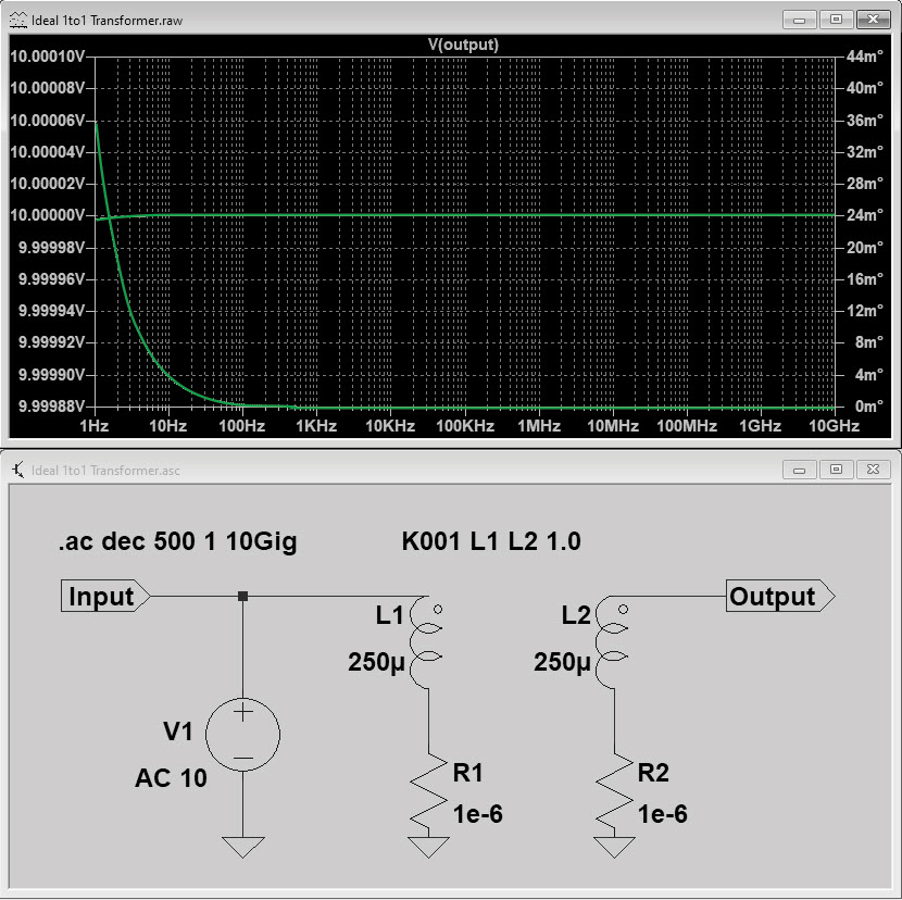
For example, a basic 1:1 ideal transformer model can be made by creating two equal inductors and assigning a perfect coupling factor of 1.0. Figure 1 shows a simulation of 10 V output at 10 V input across an extremely wide frequency band for a 1:1 250 µH ideal transformer. If the midband insertion loss of the real transformer is known to be low enough at the operating frequency, this ideal model can be functional in a circuit simulation. However, a more realistic model includes the coil DC resistance (DCR) and non-ideal coupling, which can be modeled by either leakage inductance or a coupling factor.

Doc1709_Fig1-Ideal-Voutput-Transformer.jpg
Figure 1: Ideal transformer with perfect coupling

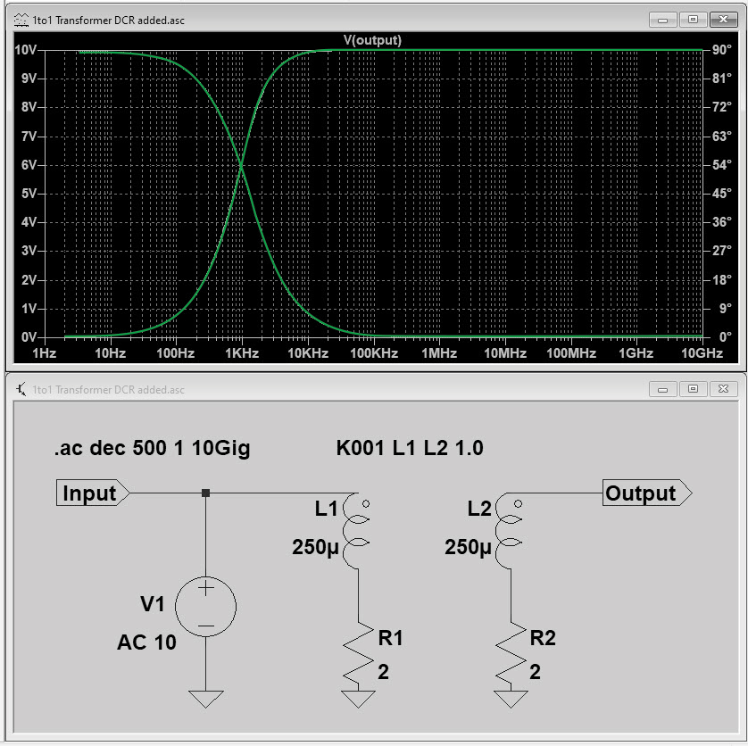
Doc1709_Fig2-Adding-DCR-model.jpg
Figure 2: Model of Figure 1 with DCR added

Effects of Including DCR and Leakage Inductance

The low-frequency cut-off of a transformer is determined by the primary magnetizing inductance in series with the primary DCR. Figure 2 shows the effect of adding the DCR of the windings (compare to Figure 1). When leakage inductance or a coupling factor <1 is not included in the model, the high-frequency cutoff is not simulated. If the leakage inductance is not published, well-designed transformers typically have worst-case leakage inductance (Lleakage) of approximately 3% of the primary L value.

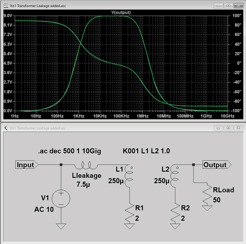
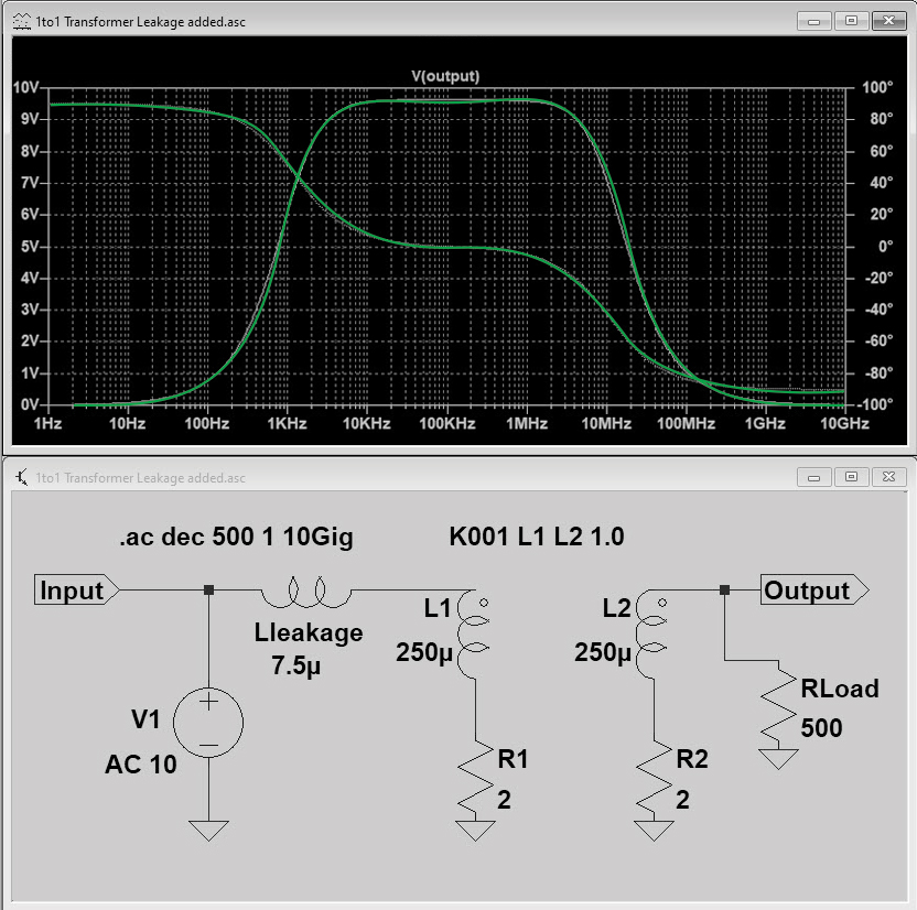
Leakage inductance is related to the coupling coefficient (K) in the following manner: Lleakage = L * (1-K^2). Figure 3 shows the effect of adding leakage inductance, which equates to a non-ideal coupling coefficient: The upper-frequency cutoff is now visible. A 50 Ohm resistance was also added to simulate a load on the output. The addition of leakage inductance and load resistance highlights the high frequency cutoff. It also shows a drop in Vout to 9 V (at best) over the 10 kHz ~ 150 kHz range. Now we are only showing 9 V output from what we thought was a 10 Vout transformer. Why does this transformer look so bad in simulation?

As seen in Figure 4, increasing the load resistance from 50 to 500 Ohms improves (reduces) the insertion loss and widens the usable bandwidth. This highlights the sensitivity of transformer bandwidth to load impedance. If the transformer is capable of sourcing the higher current drawn by the 50 Ohm load, the usable bandwidth is decreased at that load. This is a powerful illustration of the effect of load impedance on transformer efficiency. When using transformer models in time-domain simulations, this conclusion is not so obvious.

With the 50 Ohm, high-current load, the “10V” transformer is only capable of outputting 9V maximum, assuming operation is within the 10 to 150 kHz range. Higher frequency operation will show an even lower Vout. Therefore, simulation is most meaningful when the simulated load resistance (and reactance) is close to matching the actual load the transformer will see in the application. With Vout and the approximate output power of the transformer known, the load resistance can be estimated as Rload = Vout^2/Pout.

Doc1709_Fig3-Adding-leakageL-Load-R-tif.jpg
Figure 3: Effects of leakage inductance and load resistance

Doc1709_Fig4-Increasing-Load-Resistance.jpg
Figure 4: Effects of increased load resistance

Step-up and Step-down Transformers

When modeling step-up or step-down transformers, the inductance of the secondary is calculated by the sec : pri turns ratio squared times the primary inductance. When analyzing the bandwidth of step-up or step-down transformers, connect two of the transformer models back-to-back to get the impedance-matched results. When analyzing insertion loss, remember to divide the results by two, because two transformers are being simulated.

Transformers in Power Supply Simulations

When using transformers in switched-mode power supply simulations at typical kHz frequencies, ignoring the leakage inductance simplifies the model. When adding leakage inductance to the model, any capacitance that may resonate with it should be included, along with any resistive losses that limit the peak of the resonance. This complicates the model significantly. It is not too difficult to measure the primary, secondary, and primary-to-secondary capacitances, however modeling the resistive loss that limits the resonance peak(s) can be a major challenge when accurate parasitics are not known. For this reason, avoid adding leakage inductance or capacitances to the model when not using the simulation to explore bandwidth or other high-frequency effects, such as analyzing ringing for a snubber circuit design.

Current Sense Transformer Models

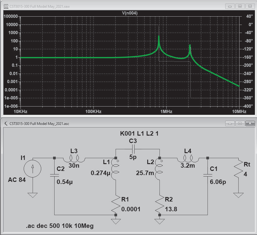
Current sense transformer models are similar to voltage transformer models in that the capacitive elements can show ringing in the simulation that is not seen in a real measurement of output voltage vs input current. For example, Figure 5 shows a simulation of Coilcraft CST3015-300L based on measurements of the individual lumped element L, C, and R parameters. The model does not include elements to capture the loss that limits ringing, and when added, still does not predict the correct linear range of the transformer. In fact, the measured usable bandwidth of this current transformer is well beyond that predicted by this model. When the real transformer is measured for Vout vs input current, the performance is linear beyond 1 MHz. As with voltage transformers, avoid adding leakage inductance or capacitance to the model unless the model is validated with input current vs output voltage measurements.

Transformer Saturation Models

While saturation models, like the Chan model, are interesting, they require proprietary material information that transformer manufacturers do not publish in order to protect their intellectual property. Traditional high-frequency power transformers are constructed with ferrite cores having hard-saturation characteristics. This means the slope of the inductance vs current curve is steep, so a small error in the model can result in a large error in simulation. Unless the model factors in variation in inductance due to core material tolerances, it could lead to false conclusions in the saturation region if it is not centered on the inductance distribution. For these reasons, unless the operating point is close to saturation, a non-saturating model is advised.

Doc1709_Fig5-Measured-Parameter-Model.jpg
Figure 5. Coilcraft CST3015-300L Measured Parameter Model

Modeling Transformer Loss for an Efficiency Analysis

When using transformer models for loss or efficiency analysis, the model must capture current-dependent and frequency-dependent loss. Traditional models that use a fixed-value parallel resistor to model core loss do not capture frequency-dependent (AC) loss. Even when a frequency-dependent parallel resistor is used, this type of model often has poor correlation with real measurements of core loss at higher current.

The Steinmetz equation is typically employed to describe the flux-density- and frequency-dependence of core loss. Core manufacturers curve-fit measurements to facilitate calculations of core loss over a range of operating conditions. As evidenced by various core material loss curves, the Steinmetz equation is only useful over a narrow range of frequencies. Therefore, a single Steinmetz equation for core loss does not fully capture all operating conditions\ and ignores conductor losses.

While the brightest minds in magnetics are working to develop improved loss models, a universal inductor SPICE model that captures all AC loss mechanisms (core loss, skin effect, proximity effect, radiation) does not yet exist. Physics-based models for capturing such loss mechanisms appear to be on the horizon, however, a practical model is not yet available to transformer manufacturers.

Coilcraft Transformer Models

Coilcraft has not published SPICE models for transformers, however, we are happy to support our customers in model-development and simulation efforts. 

Contact us to discuss your specific transformer simulation and loss calculation requirements.

Conclusion

Simulating power transformers in SPICE can provide pre-prototyping insights about in-circuit functional (or non-functional) performance. Simple coupled-inductor models are often sufficient when used near the functional mid-band frequency of the transformer and under non-extreme operating conditions. Advanced models are challenging, as the interaction of inductive, capacitive, and resistive parasitics must be knowledgeably modeled and verified. Any proposed model should be validated with end-application measurements for improved confidence in the simulations.